Case study: sparse factors in S&P 500 returns • msPCA

This vignette works through a complete, non-trivial application of msPCA to financial return data. It illustrates the practical difference between the two notions of non-redundancy that the package supports —orthogonal loadings and uncorrelated principal components— and shows that the choice materially changes the factors you recover.

Every msPCA result below reproduces from data shipped with the package: no downloads, no accounts, no external files. The fitting chunks are marked eval = FALSE only to keep the vignette quick to build (the full sparsity grid takes several minutes). Note that the benchmark method,
nsprcomp needs a data matrix rather than a correlation matrix.

The data

The dataset snp500 is the market-deflated correlation matrix of daily log-returns for p = 423 S&P 500 constituents with complete price histories from January 2010 to December 2019 (n = 2,515 trading days).

library("msPCA")
data(snp500)

dim(snp500)
#> [1] 423 423
round(snp500[1:4, 1:4], 3)
#>           A   AAPL   ABT   ACGL
#> A     0.433  0.004 0.031 -0.027
#> AAPL  0.004  0.716 0.012 -0.048
#> ABT   0.031  0.012 0.614  0.010
#> ACGL -0.027 -0.048 0.010  0.631

The matrix was constructed from the S&P 500 daily update dataset on Kaggle, released under CC0 1.0. Typically, stock returns are dominated by a “market factor” that absorbs a disproportionate share of total variance. To expose cross-sectional structure (sector and style effects) rather than market-wide movements, we projected out the leading eigenvector $v_1$ of the empirical correlation matrix $\Sigma$ , so $\texttt{snp500} = P^\top \Sigma P$ with $P = I - v_1 v_1^\top$ . The matrix is rank $p - 1=422$ :

ev <- eigen(snp500, symmetric = TRUE, only.values = TRUE)$values
sum(ev > 1e-8)          # 422: the market direction has been removed
#> [1] 422

The full data processing script is provided in data-raw/snp500.R in the package repository, and ?snp500 documents the format.

Sparse factor extraction

We extract r = 4 sparse factors, each allowed to load on at most k stocks, varying k from 5 to 35 in steps of 5 and running the analysis under both constraint types. The code below produces the results for the orthogonality constraint (feasibilityConstraintType = 0); setting feasibilityConstraintType = 1 gives the zero pairwise correlation results.

ks_grid <- seq(5, 35, by = 5)

results <- lapply(ks_grid, function(k) {
  set.seed(42)
  res <- mspca(snp500, r = 4, ks = rep(k, 4), verbose = FALSE,
               maxIter = 100, feasibilityConstraintType = 0)
  data.frame(
    k      = k,
    fve    = fraction_variance_explained(snp500, res$x_best),
    orth   = feasibility_violation_off(snp500, res$x_best, 0),
    pwcorr = feasibility_violation_off(snp500, res$x_best, 1)
  )
})
results_df <- do.call(rbind, results)

We also run nsprcomp::nsprcomp() (Sigg 2019) at the same budgets as a reference. Note that nsprcomp() requires a data matrix rather than a covariance matrix, so it needs the deflated returns XR <- X %*% P rather than snp500. That matrix is 2,515 x 423 and is not shipped with the package; data-raw/snp500.R documents how to rebuild it from the raw prices. We include a pre-computed comparison instead here, so the numbers below can be inspected and re-plotted without a rerun:

res_grid <- read.csv(system.file("vignette-data", "snp_varyingk_results.csv",
                                 package = "msPCA"))

ks  <- sort(unique(res_grid$k))
by_constraint <- function(cn) {
  sub <- res_grid[res_grid$constraint == cn, ]
  sub[match(ks, sub$k), c("fve", "orth_violation")]
}

tab <- cbind(k = ks,
             by_constraint("orthogonality"),
             by_constraint("zero-correlation"),
             by_constraint("nsprcomp"))

knitr::kable(
  tab, digits = 4, row.names = FALSE,
  col.names = c("k", "FVE (msPCA - orth)", "orth viol (msPCA - orth)", "FVE (msPCA - zero-corr)",
                "orth viol (msPCA - zero-corr)", "FVE (nsprcomp)", "orth viol (nsprcomp)"),
  caption = paste("FVE and orthogonality violation across the sparsity grid.",
                  "Every violation column reports the orthogonality violation,",
                  "including for the fits run under the zero-correlation constraint.")
)

FVE and orthogonality violation across the sparsity grid. Every violation column reports the orthogonality violation, including for the fits run under the zero-correlation constraint.
k	FVE (msPCA - orth)	orth viol (msPCA - orth)	FVE (msPCA - zero-corr)	orth viol (msPCA - zero-corr)	FVE (nsprcomp)	orth viol (nsprcomp)
5	0.0347	0.0155	0.0250	0.2331	0.0417	0.0000
10	0.0639	0.0001	0.0383	0.3327	0.0660	0.0000
15	0.0758	0.0001	0.0493	0.3470	0.0832	0.0000
20	0.0930	0.0001	0.0596	0.2998	0.0986	0.0000
25	0.0953	0.0001	0.0658	0.2780	0.1083	0.0148
30	0.1113	0.0001	0.0783	0.4033	0.1025	0.1168
35	0.1142	0.0001	0.0795	0.3180	0.1051	0.2349

Comparing the two constraint types

The figures below report the fraction of variance explained (FVE), the orthogonality violation, and the uncorrelatedness violation as a function of k, for msPCA under each constraint type, against nsprcomp::nsprcomp() at the same sparsity budgets.

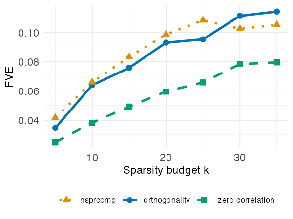
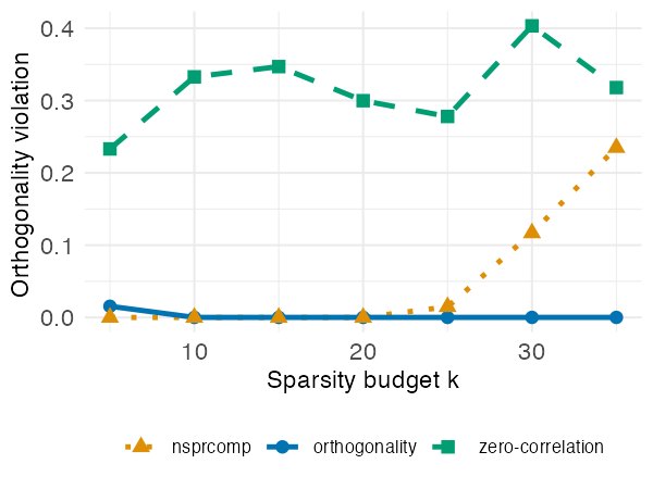
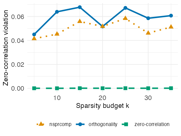
Left: fraction of variance explained vs. sparsity budget k. Center: orthogonality violation vs. k. Right: uncorrelatedness violation vs. k. Results are shown for msPCA with orthogonality constraints (blue, solid), msPCA with zero pairwise correlation constraints (green, dashed), and nsprcomp::nsprcomp() (orange, dotted). All methods use r = 4 components.

On this dataset, nsprcomp::nsprcomp() returns exactly orthogonal loading vectors for small-to-moderate sparsity budgets (k <= 20), reflecting the effectiveness of the deflation procedure when component supports can easily be disjoint. Beyond that orthogonality breaks down, and does so steeply: the violation is 0.015 at k = 25, 0.12 at k = 30 and 0.23 at k = 35.

By contrast, msPCA with orthogonality constraints holds the violation at or below 1e-4 — the default feasibility tolerance — at every budget from k = 10 upward, because the penalty on constraint violation is explicitly tightened throughout the algorithm. In terms of FVE the two methods are comparable, with a small edge for nsprcomp::nsprcomp() up to k = 25. At k = 30 and k = 35 — precisely the budgets where nsprcomp::nsprcomp() gives up orthogonality — msPCA overtakes it, reaching an FVE of 0.111 and 0.114 against 0.102 and 0.105 while keeping the violation below tolerance.

Neither nsprcomp::nsprcomp() nor orthogonality-constrained msPCA yields uncorrelated PCs here. To obtain uncorrelated PCs we run msPCA with pairwise correlation constraints instead, which yields PCs with near-zero pairwise correlation that are not mutually orthogonal. On this dataset, requiring zero pairwise correlation rather than orthogonality is possible only at the expense of a substantially lower FVE.

The two constraints correspond to different feasibility definitions and lead to meaningfully different factor compositions. msPCA lets the user choose and enforce whichever is relevant to their use case, with predictable behavior across the full range of sparsity levels.

Interpreting the sparse components

Fixing k = 10, each factor loads on 10 stocks out of 423, making it possible to associate each component with an economic theme. Sector labels below follow the Global Industry Classification Standard [GICS; MSCI and S&P Dow Jones Indices (2023)].

set.seed(42)
res_orth <- mspca(snp500, r = 4, ks = rep(10, 4), verbose = FALSE,
                  maxIter = 100, feasibilityConstraintType = 0)
set.seed(42)
res_corr <- mspca(snp500, r = 4, ks = rep(10, 4), verbose = FALSE,
                  maxIter = 100, feasibilityConstraintType = 1)

print(res_orth)
print(res_corr)

summary() on either fit reports the violations under the constraint that fit enforced, and labels them as such:

summary(res_orth)
summary(res_corr)

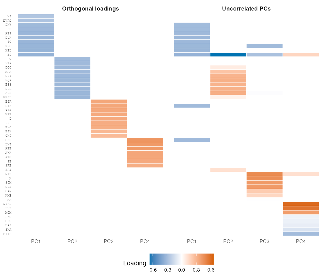
Loadings of the 4 PCs (sparsity k = 10) returned by msPCA with orthogonality (left) or zero-correlation (right) constraints.

Under orthogonality constraints

The four PCs concentrate entirely within the utility and REIT sectors, with no cross-sector loadings. Each PC has 10 nonzeros by construction, but a few are numerically negligible (below 1e-4); the economically meaningful names are:

PC1 loads on regulated electric utilities (AEP, DUK, ED, ES, EVRG, NI, PNW, SO, WEC, XEL).
PC2 consolidates the REIT segment into a single component spanning residential apartments (AVB, CPT, EQR, ESS, MAA, UDR), healthcare REITs (DOC, WELL, VTR), and net-lease (O).
PC3 captures a second, non-overlapping utility cluster (CNP, D, DTE, EIX, ETR, EXC, NEE, PEG, PPL).
PC4 identifies a third utility subgroup (AEE, ATO, AWK, CMS, FE, LNT, SRE).

The orthogonality constraint therefore fragments the market into three disjoint utility clusters and one diversified REIT basket, with each PC loading exclusively on one sector. The four components carry comparable weight, explaining 2.13%, 1.62%, 1.52% and 1.21% of total variance respectively.

Under zero-correlation constraints

The components are more sector-diverse, and their supports overlap rather than partitioning the universe — Consolidated Edison (ED) appears in all four. Variance is also far more concentrated in the leading component: 2.28%, 0.64%, 0.63% and 0.45%, against a much flatter profile under orthogonality.

PC1 consolidates the entire utility sector into a single broad component (AEP, CMS, DTE, DUK, ED, ES, PNW, SO, WEC, XEL, all loading between -0.30 and -0.34), merging stocks that the orthogonality constraint split across three separate PCs.
PC2 is a REIT component set against a single utility: residential apartment REITs (AVB, EQR, UDR, ESS, CPT at 0.30–0.33, MAA at 0.24) together with retail (FRT, 0.12) and healthcare REITs (DOC, 0.08; WELL, 0.05), against ED at -0.65.
PC3 identifies packaged food and household staples —General Mills (GIS, 0.47), Kellanova (K, 0.45), Smucker (SJM, 0.41), Campbell’s (CPB, 0.41), Conagra (CAG, 0.21) and Kimberly-Clark (KMB, 0.16)— against the utilities WEC (-0.31) and ED (-0.28).
PC4 is a casino and resort component: Wynn (WYNN) and Las Vegas Sands (LVS) load at 0.60 and 0.56, MGM at 0.40, with ED at 0.16 and GIS at 0.12, against Biogen (BIIB) at -0.30 and smaller negative loadings on Snap-on (SNA), UPS, Genuine Parts (GPC) and Packaging Corporation (PKG).

Signs are arbitrary up to a global flip within each component; what matters is the contrast between the positively and negatively loaded groups.

Takeaway

Orthogonality and zero pairwise correlation are not interchangeable. On strongly correlated data they recover qualitatively different factor structures. On this stock return data, orthogonality returns disjoint supports and spends all four components inside two sectors: three separate utility clusters and one REIT basket. Zero pairwise correlation, on the other hand, returns overlapping supports and recovers four distinct themes instead —utilities, REITs, packaged food and household staples, and casino operators— each expressed as a contrast between positively and negatively loaded groups. We also observe a difference in the distribution of variance explained by each PC: under zero correlation the leading component carries most of the explained variance (2.28% against 0.45–0.64% for the others), whereas orthogonality spreads it more evenly (2.13% down to 1.21%), and total FVE is markedly lower with zero-correlation constraints at every sparsity budget.

References

MSCI, and S&P Dow Jones Indices. 2023. The Global Industry Classification Standard (GICS). Https://www.msci.com/our-solutions/indexes/gics.

Sigg, Christian D. 2019. nsprcomp: Non-Negative and Sparse PCA. https://CRAN.R-project.org/package=nsprcomp.