Sparse PCA with multiple principal components in R.
The msPCA package computes sparse loading vectors that explain a high fraction of variance while controlling non-redundancy across components. It supports two non-redundancy definitions:
- orthogonality of loading vectors,
- zero pairwise correlation of components.
Installation
Install from CRAN:
install.packages("msPCA")
library(msPCA)
Install development version from GitHub:
install.packages("devtools")
devtools::install_github("jeanpauphilet/msPCA")
library(msPCA)
Quick start
The main function is mspca().
Inputs (following the elasticnet convention, the data is a single argument M plus a type selector):
-
M: the data matrix, -
type:"Sigma"(default) treatsMas a covariance/correlation matrix (p x p);"X"treatsMas a raw data matrix (nobservations xpvariables), -
r: number of sparse principal components, -
ks: integer vector of lengthrwith sparsity budgets.
With type = "X", mspca() applies the algorithm to the data directly via the products t(X) %*% (X %*% beta) and never forms the p x p matrix. This is substantially faster and more memory-efficient when n << p. Pass type = "X" whenever the number of variables greatly exceeds the number of observations.
Output fields:
-
x_best: sparse loading matrix (p x r), -
objective_value, -
feasibility_violation, -
runtime.
Example on mtcars:
library(msPCA)

Sigma <- cor(datasets::mtcars)
set.seed(42)

res <- mspca(Sigma, r = 2, ks = c(4, 4), verbose = FALSE)   # type = "Sigma" is the default
print_mspca(res, Sigma)

feasibility_violation_off(Sigma, res$x_best, feasibilityConstraintType = 0)
fraction_variance_explained(Sigma, res$x_best)
Equivalent workflow from the raw data matrix (no covariance matrix needed):
library(msPCA)

X <- as.matrix(datasets::mtcars)
set.seed(42)

# type = "X" treats the first argument as raw data; scale = TRUE operates on the
# correlation matrix, matching cor(mtcars) above.
res <- mspca(X, r = 2, ks = c(4, 4), type = "X", scale = TRUE, verbose = FALSE)
print_mspca(res)                      # type = "X" results carry their own variance summary

fraction_variance_explained(cor(X), res$x_best)
For datasets with n << p, this raw-data path avoids the O(np^2) cost of forming Sigma and reduces each iteration’s matrix–vector product from O(p^2) to O(np).
Optional dense PCA comparison:
pca_res <- prcomp(datasets::mtcars, scale. = TRUE)
fraction_variance_explained(Sigma, pca_res$rotation[, 1:2])
Interpretation:
- Dense PCA usually explains more variance.
- Sparse PCA improves interpretability by restricting each component to a small set of features.
See vignette("msPCA") for a worked example built from the same mtcars workflow.
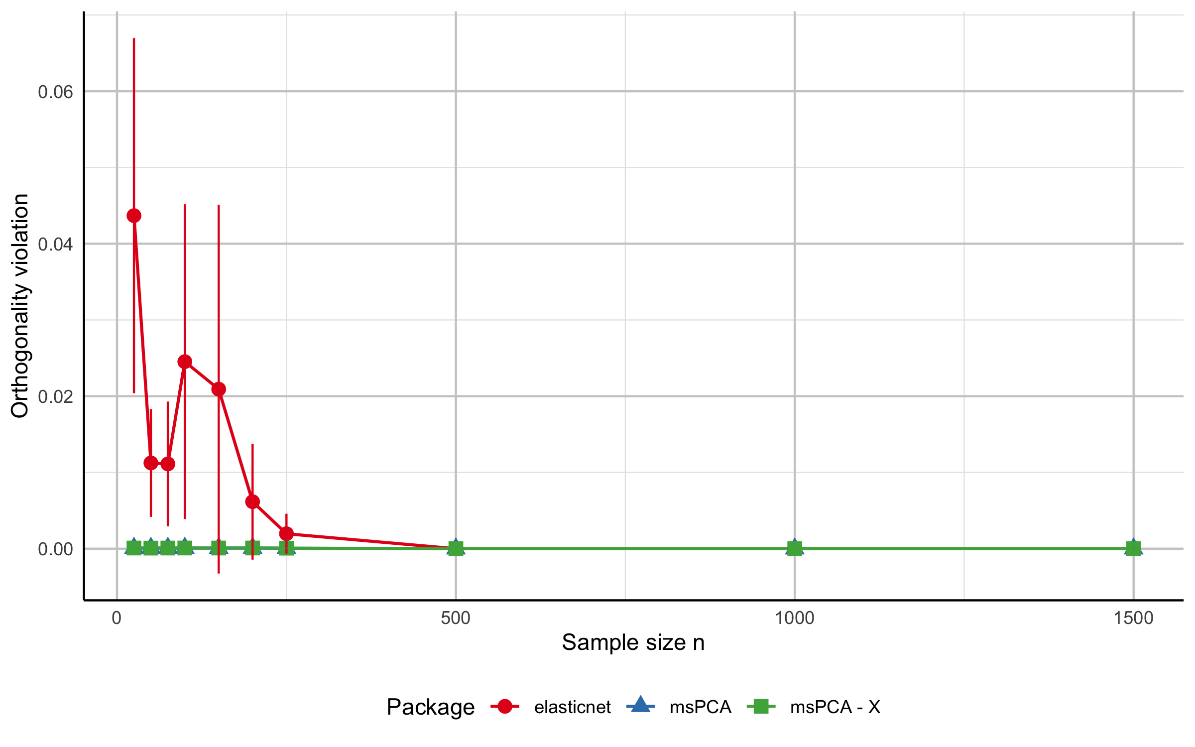
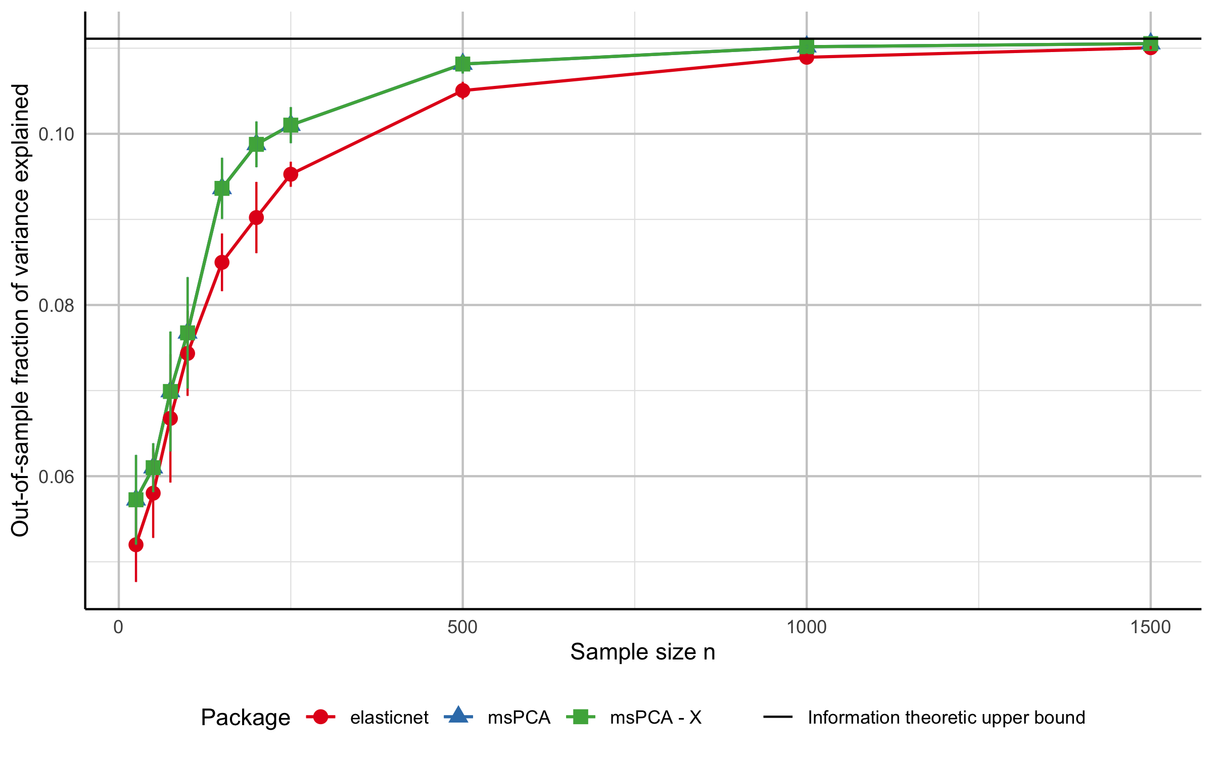
Synthetic benchmark
The script test/notebook_synthetic.R compares msPCA with elasticnet::spca() on synthetic data across sample sizes and exports the figures below.
To regenerate these files, run test/notebook_synthetic.R from the repository root.
Choosing parameters
Sparsity budgets (ks)
ks is the main tuning input. A practical workflow is to run mspca() for multiple sparsity budgets and evaluate:
- fraction of variance explained (
fraction_variance_explained()), - feasibility violation (
feasibility_violation_off()), - interpretability of nonzero loadings.
Main functions
-
mspca(M, r, ks, type = c("Sigma", "X"), ...): multiple sparse PCs. -
tpm(M, k, type = c("Sigma", "X"), ...): single sparse PC via truncated power method.
Useful optional arguments in mspca():
feasibilityConstraintTypefeasibilityTolerancemaxIterstallingTolerancetimeLimitTPMmaxRestartTPMminRestartTPM
Raw-data arguments (type = "X"):
-
center(defaultTRUE),scale(defaultTRUE, setFALSEfor covariance), -
divisor("n-1"for the sample covariance, the default, or"n").
Covariance-matrix validation arguments (type = "Sigma"):
-
checkPSD(defaultTRUE),symTolerance,psdTolerance.
Diagnostic functions
fraction_variance_explained(Sigma, U)fraction_variance_explained_perPC(Sigma, U)variance_explained_perPC(Sigma, U)feasibility_violation_off(Sigma, U, feasibilityConstraintType)print_mspca(sol_object, Sigma, digits = 3)
Citation
If you use msPCA in academic work, please cite the package and the underlying paper.
You can retrieve the package citation in R with:
citation("msPCA")Reference paper:
Development
Package structure overview:
-
R/-
main.R: user-facing functions and helper diagnostics. -
RcppExports.R: R interface for compiled code (typically generated withRcpp::compileAttributes()).
-
-
src/-
msPCA_R_CPP.cpp: C++ implementation of the core algorithm and the dense/raw-data entry points. -
CovOperator.h: covariance-operator abstraction (DenseOpforSigma,GramOpforX). -
ConstantArguments.h: internal algorithm constants. -
RcppExports.cpp: generated C++ interface. -
Makevars,Makevars.win: compilation settings.
-
-
man/: function documentation generated from roxygen comments. -
test/notebook_mtcars.Rnotebook_plot.Rnotebook_synthetic.RmsPCA_synthetic_results.csv
For interface changes, regenerate exports and documentation with Rcpp::compileAttributes() and devtools::document().